ESTIA advanced data reduction

• Audience: Instrument (data) scientists, instrument users

• Prerequisites: Basic knowledge of Scipp, Sciline

This notebook builds on the basic ESTIA reduction guide; you should read that first. This advanced guide demonstrates how the workflow can be used to make diagnostics plots and options for processing multiple files together. e the default loader with the load_mcstas_events provider.

The data is available through the ESSreflectometry package but accessing it requires the pooch package. If you get an error about a missing module pooch, you can install it with !pip install pooch.

from typing import NewType

import pandas as pd
import sciline
import scipp as sc

from ess.estia.data import estia_mcstas_example, estia_mcstas_groundtruth
from ess.estia import EstiaMcStasWorkflow
from ess.reflectometry.types import *
from ess.reflectometry.figures import wavelength_z_figure, wavelength_theta_figure, q_theta_figure

Process multiple files

To apply the ESTIA workflow to multiple files, we could simply write a for-loop like this:

results = []
for filename in estia_mcstas_example('Ni/Ti-multilayer'):
    wf[Filename[SampleRun]] = filename
    results.append(wf.compute(ReflectivityOverQ))

However, this would re-load and re-process the reference measurement for every sample file. Instead, we will use Sciline’s map-reduce feature to map the workflow over several files and merge the individual results.

First, we set up the workflow in almost the same way as in the basic ESTIA reduction guide, except that we do not set a filename for the sample run.

wf = EstiaMcStasWorkflow()
wf[Filename[ReferenceRun]] = estia_mcstas_example('reference')

wf[YIndexLimits] = sc.scalar(35), sc.scalar(64)
wf[ZIndexLimits] = sc.scalar(0), sc.scalar(48 * 32)
wf[BeamDivergenceLimits] = sc.scalar(-0.75, unit='deg'), sc.scalar(0.75, unit='deg')

wf[WavelengthBins] = sc.geomspace('wavelength', 3.5, 12, 2001, unit='angstrom')
wf[QBins] = 1000

# There is no proton current data in the McStas files, here we just add some fake proton current
# data to make the workflow run.
wf[ProtonCurrent[SampleRun]] = sc.DataArray(
    sc.array(dims=('time',), values=[]),
    coords={'time': sc.array(dims=('time',), values=[], unit='s')})
wf[ProtonCurrent[ReferenceRun]] = sc.DataArray(
    sc.array(dims=('time',), values=[]),
    coords={'time': sc.array(dims=('time',), values=[], unit='s')})

Downloading file 'examples/220573/mccode.h5' from 'https://public.esss.dk/groups/scipp/ess/estia/1/examples/220573/mccode.h5' to '/home/runner/.cache/ess/estia/1'.

Reflectivity vs. Q

In this section, we compute the reflectivity as a function of momentum transfer for a number of files with the same sample at different sample rotations. We will map the workflow over the ames for each file and reduce the results into a single data group.

Starting with a parameter table of filenames, we map the workflow:

param_table = pd.DataFrame({
    Filename[SampleRun]: estia_mcstas_example('Ni/Ti-multilayer')
}).rename_axis(index='sample_rotation')

# Make a copy to preserve the original `wf`.
multi_file_workflow = wf.copy()
mapped = multi_file_workflow[ReflectivityOverQ].map(param_table)

Downloading file 'examples/220574/mccode.h5' from 'https://public.esss.dk/groups/scipp/ess/estia/1/examples/220574/mccode.h5' to '/home/runner/.cache/ess/estia/1'.
Downloading file 'examples/220575/mccode.h5' from 'https://public.esss.dk/groups/scipp/ess/estia/1/examples/220575/mccode.h5' to '/home/runner/.cache/ess/estia/1'.
Downloading file 'examples/220576/mccode.h5' from 'https://public.esss.dk/groups/scipp/ess/estia/1/examples/220576/mccode.h5' to '/home/runner/.cache/ess/estia/1'.
Downloading file 'examples/220577/mccode.h5' from 'https://public.esss.dk/groups/scipp/ess/estia/1/examples/220577/mccode.h5' to '/home/runner/.cache/ess/estia/1'.

Then we merge the reflectivity data for all files into a single data group. We use the sample rotation as key because in this example, each file contains data at a different rotation.

def combine_measurements(*measurements: sc.DataArray) -> sc.DataGroup[sc.DataArray]:
    return sc.DataGroup({
        f"{da.coords['sample_rotation']:c}": da for da in measurements
    })

multi_file_workflow[ReflectivityOverQ] = mapped.reduce(
    func=combine_measurements
)

The graph now indicates that everything that depends on SampleRun data has been mapped: (Names shown in boxes as opposed to rectangles have been mapped.)

multi_file_workflow.visualize(
    ReflectivityOverQ,
    graph_attr={"rankdir": "LR"},
    compact=True,
)

We compute the reflectivity for each file and get a data group:

reflectivities = multi_file_workflow.compute(ReflectivityOverQ)
reflectivities

scipp.DataGroup

(Q: 1000)

• 1.0 deg

  scipp

  DataArray

  (Q: 1000)

  float64

  𝟙

  binned data [len=3, len=3, ..., len=0, len=2]
• 2.0 deg

  scipp

  DataArray

  (Q: 1000)

  float64

  𝟙

  binned data [len=3, len=2, ..., len=0, len=1]
• 4.0 deg

  scipp

  DataArray

  (Q: 1000)

  float64

  𝟙

  binned data [len=1, len=1, ..., len=5, len=2]
• 8.0 deg

  scipp

  DataArray

  (Q: 1000)

  float64

  𝟙

  binned data [len=5, len=2, ..., len=1, len=2]

reflectivities.hist().plot(norm='log', vmin=1e-8)

/home/runner/work/essreflectometry/essreflectometry/.tox/docs/lib/python3.10/site-packages/matplotlib/axes/_axes.py:3828: RuntimeWarning: invalid value encountered in add
  low, high = dep + np.vstack([-(1 - lolims), 1 - uplims]) * err

Reflectivity vs. Q with custom mask

The data is very noisy in some \(Q\) bins. We can clean up the plot by removing or masking those bins. The variance of the reference measurement is a good measure for how noisy the final data will be, so we use that to insert a mask into the reflectivity curve. This means that we need to request Reference to construct the mask. But since the value of Reference is different for each sample run, we need to insert a new step into the workflow and include it in the map-operation. See also Replacing providers for a more general guide.

We define a custom type (MaskedReflectivityOverQ) and a provider to apply the mask:

MaskedReflectivityOverQ = NewType('MaskedReflectivityOverQ', sc.DataArray)

def mask_noisy_reference(
    reflectivity: ReflectivityOverQ,
    reference: Reference,
) -> MaskedReflectivityOverQ:
    ref = reference.hist(Q=reflectivity.coords['Q'])
    return reflectivity.assign_masks(
        noisy_reference= sc.stddevs(ref).data > 0.3 * ref.data
    )

wf.insert(mask_noisy_reference)

Note that the code above inserts into wf, i.e., the unmapped workflow. Now map-reduce the workflow again but in the new MaskedReflectivityOverQ type:

multi_file_workflow = wf.copy()
param_table = pd.DataFrame({
    Filename[SampleRun]: estia_mcstas_example('Ni/Ti-multilayer')
}).rename_axis(index='run')
mapped = multi_file_workflow[MaskedReflectivityOverQ].map(param_table)
multi_file_workflow[MaskedReflectivityOverQ] = mapped.reduce(
    func=combine_measurements
)

The graph is the same as before except that only MaskedReflectivityOverQ is available as a final, unmapped type:

multi_file_workflow.visualize(
    MaskedReflectivityOverQ,
    graph_attr={"rankdir": "LR"},
    compact=True,
)

Compute the results:

reflectivities = multi_file_workflow.compute(MaskedReflectivityOverQ)
reflectivities

scipp.DataGroup

(Q: 1000)

• 1.0 deg

  scipp

  DataArray

  (Q: 1000)

  float64

  𝟙

  binned data [len=3, len=3, ..., len=0, len=2]
• 2.0 deg

  scipp

  DataArray

  (Q: 1000)

  float64

  𝟙

  binned data [len=3, len=2, ..., len=0, len=1]
• 4.0 deg

  scipp

  DataArray

  (Q: 1000)

  float64

  𝟙

  binned data [len=1, len=1, ..., len=5, len=2]
• 8.0 deg

  scipp

  DataArray

  (Q: 1000)

  float64

  𝟙

  binned data [len=5, len=2, ..., len=1, len=2]

To plot, we histogram and set values in masked bins to NaN to make the plot easier to read:

histograms = reflectivities.hist().apply(lambda R: R.assign(
    sc.where(
        R.masks['noisy_reference'],
        sc.scalar(float('nan'), unit=R.unit),
        R.data
    )
))

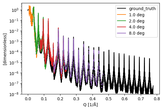
Since this data is from a McStas simulation, we know the true reflectivity of the sample. We plot it alongside the ‘measured’ reflectivity for comparison:

ground_truth = estia_mcstas_groundtruth('Ni/Ti-multilayer')
sc.plot({'ground_truth': ground_truth} | dict(histograms), norm='log', vmin=1e-8, c={'ground_truth': 'k'})

Downloading file 'examples/NiTiML.ref' from 'https://public.esss.dk/groups/scipp/ess/estia/1/examples/NiTiML.ref' to '/home/runner/.cache/ess/estia/1'.
/home/runner/work/essreflectometry/essreflectometry/.tox/docs/lib/python3.10/site-packages/matplotlib/axes/_axes.py:3828: RuntimeWarning: invalid value encountered in add
  low, high = dep + np.vstack([-(1 - lolims), 1 - uplims]) * err

Other projections

ESSreflectometry provides functions for plotting the intensity as a function of different variables. Note that these plots can also be produced by the workflow directly, see Draw diagnostics plots with the workflow. But here, we make them manually to more easily combine data from all files.

The plots consume data that is provided by the Sample key in the workflow. We could map-reduce the workflow in that key instead of in MaskedReflectivityOverQ to compute Sample for each file. But for simplicity, we use sciline.compute_mapped to compute the results for all files:

results = list(sciline.compute_mapped(multi_file_workflow, Sample))

wavelength_z_figure(results[3], wavelength_bins=400)

wavelength_theta_figure(
    results,
    wavelength_bins=200,
    theta_bins=200,
    q_edges_to_display=[sc.scalar(0.016, unit='1/angstrom'), sc.scalar(0.19, unit='1/angstrom')]
)

q_theta_figure(results, q_bins=200, theta_bins=200)

Draw diagnostics plots with the workflow

The ESTIA workflow can produce a number of plots directly to quickly visualize the data in different forms. Those plots can be combined into a single ReflectivityDiagnosticsView or constructed separately. Here, we use the combined ReflectivityDiagnosticsView but you can also request one or more of the individual views (see also the graph below):

• ReflectivityOverQ

• ReflectivityOverZW

• WavelengthThetaFigure

• WavelengthZIndexFigure

These plots correspond to the figures in the Other projections sections above but show only data from a single file.

We construct the workflow as in the basic ESTIA reduction guide but also add ThetaBins for the sample run to control the plots:

wf = EstiaMcStasWorkflow()
wf[Filename[SampleRun]] = estia_mcstas_example('Ni/Ti-multilayer')[3]
wf[Filename[ReferenceRun]] = estia_mcstas_example('reference')

wf[YIndexLimits] = sc.scalar(35), sc.scalar(64)
wf[ZIndexLimits] = sc.scalar(0), sc.scalar(48 * 32)
wf[BeamDivergenceLimits] = sc.scalar(-0.75, unit='deg'), sc.scalar(0.75, unit='deg')

wf[WavelengthBins] = sc.geomspace('wavelength', 3.5, 12, 2001, unit='angstrom')
wf[ThetaBins[SampleRun]] = 200
wf[QBins] = 1000

# There is no proton current data in the McStas files, here we just add some fake proton current
# data to make the workflow run.
wf[ProtonCurrent[SampleRun]] = sc.DataArray(
    sc.array(dims=('time',), values=[]),
    coords={'time': sc.array(dims=('time',), values=[], unit='s')})
wf[ProtonCurrent[ReferenceRun]] = sc.DataArray(
    sc.array(dims=('time',), values=[]),
    coords={'time': sc.array(dims=('time',), values=[], unit='s')})

wf.visualize(ReflectivityDiagnosticsView, graph_attr={'rankdir':'LR'})

We request the figure like any other data in the workflow:

view = wf.compute(ReflectivityDiagnosticsView)

And finally, we draw it: (this view object can be rendered in a Jupyter notebook.)

view